Geometrical spreading of sound#
As a point source extends from its origin, the intensity diminishes inversely proportional to the distance traveled, following the Inverse-square law. In the context of noise propagation, this phenomenon significantly influences the attenuation of turbine noise levels.
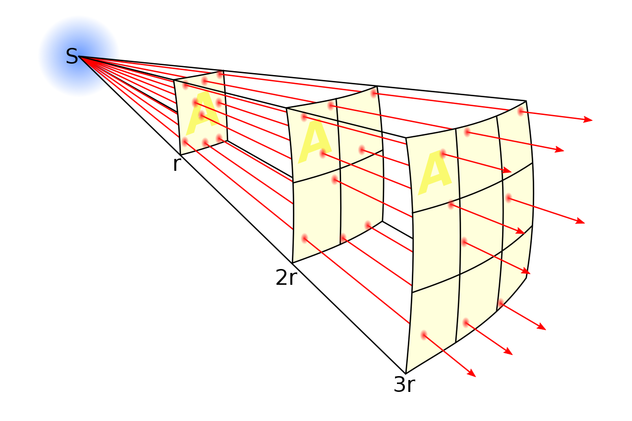
Fig 1: S denotes the noise source, and r represents the measured points. The lines illustrate noise propagation from the sources. The total noise lines, linked to source strength, remain constant, but denser lines indicate a louder noise field. The line density is inversely proportional to distance from the source squared, reflecting increased surface area on a sphere. Consequently, noise intensity inversely scales with the square of the distance from the source (Source).
Show code cell source
import numpy as np
import matplotlib.pyplot as plt
from matplotlib.animation import FuncAnimation, PillowWriter
from IPython.display import Image
Derivation#
The intensity, \(I\), measured in watts per square meter (\(W/m^2\)), is a fundamental quantity in acoustics. The sound power of a source, denoted as \(P\), can be related to intensity through the formula:
Here, \(z_0\) represents the characteristic specific acoustic impedance as is equal to \(z_0 = 400 \text{Pa} \cdot \text{s}/\text{m}\).
Rearranging the equation in terms of sound power \(P\), we get:
In the context of a reference sound power \(P_0 = 10^{-12} \text{W}\), the ratio \(\dfrac{P}{P_0}\) can be expressed as:
Where the reference sound pressure is \(p_0 = 2\cdot 10^{-5} \text{Pa}\). Taking the logarithm of both sides, we arrive at:
This expression can be further simplified to represent the sound power level as \(L_W = 10\log\left(\dfrac{P}{P_0}\right)\) and the sound pressure level as \(L_P = 10\log\left(\dfrac{p^2}{p_0^2}\right)\):
With the used reference values \(\dfrac{p_0^2}{P_0 z_0} = 1\), and the equation simplifies to:
Lastly, be rearranging the equation, the final expression for the sound pressure level can be found:
This derivation provides insights into the relationship between sound power, intensity, and their representation in logarithmic scales.
Application of function#
Utilizing the formula on a fluctuating noise signal, oscillating between 0 dB and 100 dB, reveals the impact of geometrical spreading on the noise amplitude. It’s worth mentioning that this effect is not exclusive to oscillating values; I chose to create the plot simply because of its visually interesting representation.
width = 3000  # Width of the simulation grid
height = width  # Height of the simulation grid
center_x =0 # # X-coordinate of the point source
center_y = 0 #  # Y-coordinate of the point source
frequency = 0.5 # frequency
amplitude = 100  # Amplitude of the oscillation
speed = 300  # Speed of wave propagation
duration = 3 # Duration of the simulation
fps = 10  # Frames per second
res = 500
wavelength = speed / frequency
angular_frequency = 2 * np.pi * frequency
wave_number = 2 * np.pi / wavelength

x, y = np.meshgrid(np.linspace(-width, width, res), np.linspace(-height, height, res))

fig,ax = plt.subplots()
time = 0 / fps
distance = np.sqrt((x - center_x)**2 + (y - center_y)**2)
wave = np.abs(np.maximum(0, (amplitude - 20*np.log10(distance) - 11)) * np.sin(angular_frequency * time - wave_number * distance))
cb = ax.imshow(wave, cmap='jet', origin='lower', extent=[-width, width, -height, height], vmin=0, vmax=amplitude)
plt.colorbar(cb, ax= ax, label = "SPL [dB]")
ax.set(xlabel= " X [m]",
       ylabel = "Y [m]")
plt.close()
def update(frame):
    global grid
    time = frame / fps
    distance = np.sqrt((x - center_x)**2 + (y - center_y)**2)
    wave = np.abs(np.maximum(0,(amplitude - 20*np.log10(distance) - 11)) * np.sin(angular_frequency * time - wave_number* distance))
    ax.imshow(wave, cmap='jet', origin='lower', extent=[-width, width, -height, height], vmin=0, vmax=amplitude)
animation = FuncAnimation(fig, update, frames= int(duration * fps), interval= 1/fps)

animation.save('../../temp/ripple.gif',writer=PillowWriter(fps=fps))
Image(open('../../temp/ripple.gif','rb').read())